Denoise with autoencoders

Autoencoders

An autoencoder is a NN structure used to extract a determined number of important features from data, using unsupervised learning. The idea is to learn an efficient representation of the data (i.e. encoding) that has a much smaller dimension when compared with the original data itself. The working principle is simple: one creates a symmetric neural network with an information bottleneck in the middle and trains it using the same dataset both as the input and output of the network. This way, the model learns to recreate the full data using only the small amount of information defined in the bottleneck of the neural network. Moreover, the model can be trained to be robust to the noise by artificially introducing noise in the input of the network.

The main uses of autoencoders include data compression, feature extraction, denoise, and the creation of generative models.

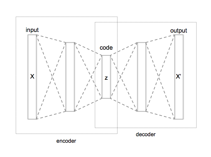
Here’s the autoencoder scheme from wiki:

Denoise application

Let’s see how one can create a simple convolutional network to encode the information of the handwritten digit following Francois Chollet’s post on his keras blog. To train the network we use the old classic mnist handwritten digits dataset (28x28x1 gray-scale images of handwritten digits):

from keras.datasets import mnist
(x_train, _), (x_test, y_test) = mnist.load_data()

x_train = x_train.astype('float32') / 255
x_test = x_test.astype('float32') / 255

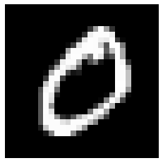
here we download the dataset directly from the keras library and we normalize the 0-255 color code. The dataset contains 60000 training and 10000 test images. Let us show a sample image from the training dataset:

import matplotlib.pyplot as plt
sample_img = x_train[1]
plt.imshow(sample_img, cmap='gray')

Training denoise autoencoder idea

To build an autoencoder for a denoise application the idea is very simple: we take an image, we add artificial noise and blurring to that image and we train the autoencoder to recover the clean image given the noisy one as input.

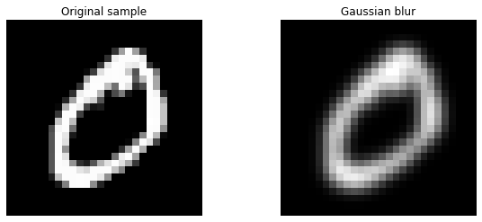
Let us start introducing a gaussian blur to our training image by using the scipy library gaussian_filter function:

from scipy import ndimage

img_blur = ndimage.gaussian_filter(sample_img, sigma=1)
fig, (ax1, ax2) = plt.subplots(1, 2, figsize=(10,4))
ax1.imshow(sample_img, cmap='gray')
ax2.imshow(img_blur, cmap='gray')

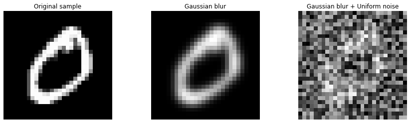
Finally, we can add a uniform noise using the numpy function random.uniform

import numpy as np

img_noise = img_blur + np.random.uniform(-1, 1, size=img_blur.shape)

fig, (ax1, ax2, ax3) = plt.subplots(1, 3, figsize=(15,4))
ax1.imshow(sample_img, cmap='gray')
ax2.imshow(img_blur, cmap='gray')
ax3.imshow(img_noise, cmap='gray')

We can write a simple helper funcion to add the noise to our training images:

def add_noise(img):
    blurring = np.random.uniform(0,2)
    img_noise = ndimage.gaussian_filter(img, sigma=blurring)
    rng = np.random.uniform(0.01,1.5)
    img_noise = img_noise + np.random.uniform(-rng, rng, size=img.shape)
    return img_noise

Here we can generate images with different noise every time, changing randomly the amount of blur and the magnitude of the uniform random noise. We finally build a generator to automatically add noise to the training images and feed the result to the fit method of our autoencoder.

import random
def Data_generator(batch_size, data_x, shuffle=True):
    data_size = len(data_x)
    index_list = [*range(data_size)]
    
    if shuffle:
        random.shuffle(index_list)
    
    index = 0
    
    while True:
        batch_x, batch_y = [], []

        for i in range(batch_size):
            if index >= data_size:
                index = 0
                if shuffle:
                    random.shuffle(index_list)

            batch_y.append(data_x[index_list[index]])
            batch_x.append(add_noise(data_x[index_list[index]]))           
        
            index += 1
        yield(np.array(batch_x), np.array(batch_y))

We can now create a training generator by selecting the training dataset and the batch size. For example, if we would like to have just two images per batch we can build the generator as follows:

train_gen = Data_generator(2, x_train)

for _ in range(2):
    img_a, img_b = next(train_gen)

    fig, (ax1, ax2, ax3, ax4) = plt.subplots(1, 4, figsize=(20,4))

    ax1.imshow(img_a[0], cmap='gray')
    ax2.imshow(img_b[0], cmap='gray')
    ax3.imshow(img_a[1], cmap='gray')
    ax4.imshow(img_b[1], cmap='gray')

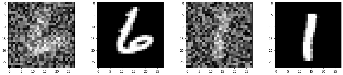
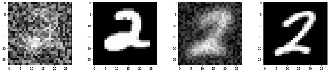
As we can see, we can loop through our generator and obtain for every loop a batch of two input and output images to train the autoencoder. The input will contain noise and blurring while the output will be clean.

Autoencoder model with tensorflow

We define the autoencoder model as follow:

from tensorflow.keras.layers import Input, Dense, Conv2D, MaxPooling2D, UpSampling2D

input_img = Input(shape=(28, 28, 1))

x = Conv2D(16, (3, 3), activation='relu', padding='same')(input_img)
x = MaxPooling2D((2, 2), padding='same')(x)
x = Conv2D(8, (3, 3), activation='relu', padding='same')(x)
x = MaxPooling2D((2, 2), padding='same')(x)
x = Conv2D(8, (3, 3), activation='relu', padding='same')(x)
encoded = MaxPooling2D((2, 2), padding='same')(x)

x = Conv2D(8, (3, 3), activation='relu', padding='same')(encoded)
x = UpSampling2D((2, 2))(x)
x = Conv2D(8, (3, 3), activation='relu', padding='same')(x)
x = UpSampling2D((2, 2))(x)
x = Conv2D(16, (3, 3), activation='relu')(x)
x = UpSampling2D((2, 2))(x)
decoded = Conv2D(1, (3, 3), activation='sigmoid', padding='same')(x)

We notice how the model is almost symmetric with respect to the middle layer (the encoded layer). The input (and output) size of the data is 784 (28*28), while the encoded representation size is (128 (4*4*8)), which is about 6 times smaller. The network is not completely symmetric because of the MaxPooling2D vs UpSampling2D layers. These two layers have no trainable parameters but they are only used to deterministically decrease (down-sampling) and increase (up-sampling) the dimension of a 2D matrix. In our example MaxPooling split the input matrix into (2x2) regions, and replaces the region with the maximum between the 4 values contained in it, shrinking the original matrix size by a factor of four. This is a convolutional operation and cannot be mathematically inverted, therefore the neural network cannot be completely symmetric. We can approximate the inversion of MaxPooling2D in different ways: one is to replace each pixel of the input image with 4 copies of it (UpSampling2D) and the second is to make the model learn the deconvolution operation as well (Conv2DTranspose). The latter option can lead to better performance but it is computationally heavier. Here, we choose to use the UpSampling2D method for its simplicity.

Model training

It is time to train the model using, for example, the adam optimizer and the binary_crossentropy as losses. To train the network we exploited the GPU runtime of (Google Colab)[colab.research.google.com], which gave us a performance boost of almost a factor of 40 compared to the standard CPU.

from tensorflow.keras.models import Model
import tensorflow as tf

autoencoder = Model(input_img, decoded)
optimizer = tf.keras.optimizers.Adam(0.003)
autoencoder.compile(optimizer=optimizer, loss='binary_crossentropy')

train_gen = Data_generator(256, x_train)
val_gen = Data_generator(256, x_test)


out = autoencoder.fit(train_gen,
                      steps_per_epoch = 230,
                      validation_data=val_gen,
                      validation_steps = 30,
                      epochs = 50,
                      verbose=1)

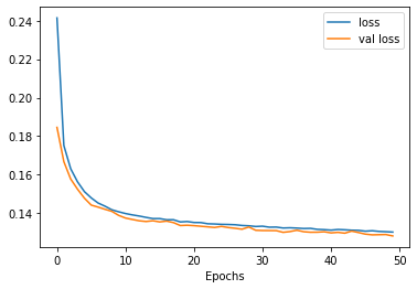
After 50 epochs of training the loss function seems to be almost saturated, without showing any overfitting issue. Adding more training time will still be beneficial for the model.

If you want to try the model without training you can download a pre-trained model from here.

Testing the model

Let’s test how the model performs on the test image dataset: we pick a random image and we feed it into the autoencoder network by progressively increasing the blurring and the noise level:

import matplotlib.pyplot as plt
fig, [ax_input, ax_output] = plt.subplots(2, 6, figsize=(12, 4))

for i in range(6):
    ax_input[i].set_xticks([])
    ax_input[i].set_yticks([])
    ax_output[i].set_xticks([])
    ax_output[i].set_yticks([])

    input_image = x_test[3].reshape(28, 28)
    input_image = ndimage.gaussian_filter(input_image, sigma=0.5*i)
    white_noise = np.random.uniform(-0.2*i,0.2*i, size=input_image.shape) * 2
    input_image = input_image + white_noise
    
    ax_input[i].imshow(input_image, cmap='gray')
    ax_input[i].set_title(f's={0.5*i:.1f}, r={0.2*i:.1f}')

    output_image = autoencoder.predict(input_image.reshape(1, 28, 28, 1))
    ax_output[i].imshow(output_image.reshape(28, 28), cmap='gray')

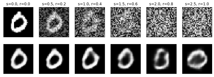
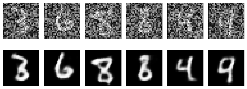
As we can see the model can drastically reduce the noise in the image, showing good results even for very high noise levels, when the digit corresponding to the input image is so blurred and noisy it cannot be identified even by humans.

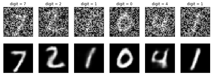
Here we plot a second example with high blurring and noise for different digits, C.S.I. yet?

fig, [ax_input, ax_output] = plt.subplots(2, 6, figsize=(12, 4))

for i in range(6):
    ax_input[i].set_xticks([])
    ax_input[i].set_yticks([])
    ax_output[i].set_xticks([])
    ax_output[i].set_yticks([])

    input_image = x_test[i].reshape(28, 28)
    input_image = ndimage.gaussian_filter(input_image, sigma=0.5*2)
    white_noise = np.random.uniform(-0.2,0.2, size=input_image.shape) * 4
    input_image = input_image + white_noise
    ax_input[i].set_title(f'digit = {y_test[i]}')
    
    ax_input[i].imshow(input_image, cmap='gray')

    output_image = autoencoder.predict(input_image.reshape(1, 28, 28, 1))
    ax_output[i].imshow(output_image.reshape(28, 28), cmap='gray')